What is Matrix in R?

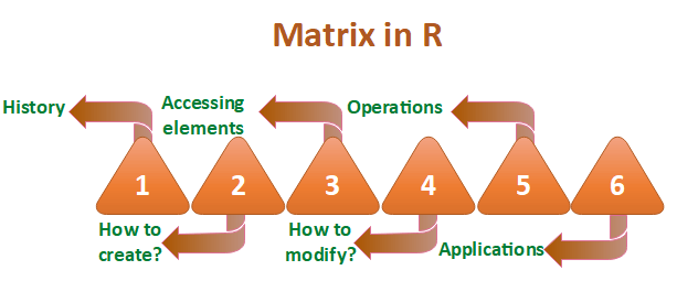
 In R, a two-dimensional rectangular data set is known as a matrix. A matrix is created with the help of the vector input to the matrix function. On R matrices, we can perform addition, subtraction, multiplication, and division operation.

In the R matrix, elements are arranged in a fixed number of rows and columns. The matrix elements are the real numbers. In R, we use matrix function, which can easily reproduce the memory representation of the matrix. In the R matrix, all the elements must share a common basic type.

Example

1. matrix1<-matrix(c(11, 13, 15, 12, 14, 16),nrow =2, ncol =3, byrow = TRUE)  
2. matrix1  

Output

[,1]  [,2]  [,3]
[1,]   11   13   15
[2,]   12   14   16

History of matrices in R

The word "Matrix" is the Latin word for womb which means a place where something is formed or produced. Two authors of historical importance have used the word "Matrix" for unusual ways. They proposed this axiom as a means to reduce any function to one of the lower types so that at the "bottom" (0order) the function is identical to its extension.

Any possible function other than a matrix from the matrix holds true with the help of the process of generalization. It will be true only when the proposition (which asserts function in question) is true. It will hold true for all or one of the value of argument only when the other argument is undetermined.

How to create a matrix in R?

Like vector and list, R provides a function which creates a matrix. R provides the matrix() function to create a matrix. This function plays an important role in data analysis. There is the following syntax of the matrix in R:

1. matrix(data, nrow, ncol, byrow, dim_name)  

data

The first argument in matrix function is data. It is the input vector which is the data elements of the matrix.

nrow

The second argument is the number of rows which we want to create in the matrix.

ncol

The third argument is the number of columns which we want to create in the matrix.

byrow

The byrow parameter is a logical clue. If its value is true, then the input vector elements are arranged by row.

dim_name

The dim_name parameter is the name assigned to the rows and columns.

Let's see an example to understand how matrix function is used to create a matrix and arrange the elements sequentially by row or column.

Example

1. #Arranging elements sequentially by row.  
2. P <- matrix(c(5:16), nrow = 4, byrow = TRUE)  
3. print(P)  
4.   
5. # Arranging elements sequentially by column.  
6. Q <- matrix(c(3:14), nrow = 4, byrow = FALSE)  
7. print(Q)  
8.   
9. # Defining the column and row names.  
10. row_names = c("row1", "row2", "row3", "row4")  
11. ccol_names = c("col1", "col2", "col3")  
12.   
13. R <- matrix(c(3:14), nrow = 4, byrow = TRUE, dimnames = list(row_names, col_names))  
14. print(R)  

Output

      [,1] [,2] [,3]
[1,]    5    6    7
[2,]    8    9   10
[3,]   11   12   13
[4,]   14   15   16

      [,1] [,2] [,3]
[1,]    3    7   11
[2,]    4    8   12
[3,]    5    9   13
[4,]    6   10   14

      col1 col2 col3
row1    3    4    5
row2    6    7    8
row3    9   10   11
row4   12   13   14

Accessing matrix elements in R

Like C and C++, we can easily access the elements of our matrix by using the index of the element. There are three ways to access the elements from the matrix.

1. We can access the element which presents on nth row and mth column.
2. We can access all the elements of the matrix which are present on the nth row.
3. We can also access all the elements of the matrix which are present on the mth column.

Let see an example to understand how elements are accessed from the matrix present on nth row mth column, nth row, or mth column.

Example

1. # Defining the column and row names.  
2. row_names = c("row1", "row2", "row3", "row4")  
3. ccol_names = c("col1", "col2", "col3")  
4. #Creating matrix   
5. R <- matrix(c(5:16), nrow = 4, byrow = TRUE, dimnames = list(row_names, col_names))  
6. print(R)  
7.   
8. #Accessing element present on 3rd row and 2nd column  
9. print(R[3,2])  
10.   
11. #Accessing element present in 3rd row  
12. print(R[3,])  
13.   
14. #Accessing element present in 2nd column  
15. print(R[,2])  

Output

      col1 col2 col3
row1    5    6    7
row2    8    9   10
row3   11   12   13
row4   14   15   16

[1] 12

col1 col2 col3
  11   12   13

row1 row2 row3 row4
   6    9   12   15

Modification of the matrix

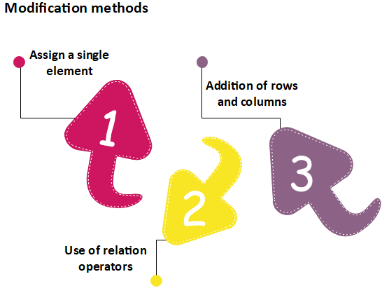
R allows us to do modification in the matrix. There are several methods to do modification in the matrix, which are as follows:

Assign a single element

In matrix modification, the first method is to assign a single element to the matrix at a particular position. By assigning a new value to that position, the old value will get replaced with the new one. This modification technique is quite simple to perform matrix modification. The basic syntax for it is as follows:

1. matrix[n, m]<-y   

Here, n and m are the rows and columns of the element, respectively. And, y is the value which we assign to modify our matrix.

Let see an example to understand how modification will be done:

Example

1. # Defining the column and row names.  
2. row_names = c("row1", "row2", "row3", "row4")  
3. ccol_names = c("col1", "col2", "col3")  
4.   
5. R <- matrix(c(5:16), nrow = 4, byrow = TRUE, dimnames = list(row_names, col_names))  
6. print(R)  
7.   
8. #Assigning value 20 to the element at 3d roe and 2nd column  
9. R[3,2]<-20  
10. print(R)  

Output

      col1 col2 col3
row1    5    6    7
row2    8    9   10
row3   11   12   13
row4   14   15   16

      col1 col2 col3
row1    5    6    7
row2    8    9   10
row3   11   20   13
row4   14   15   16

Use of Relational Operator

R provides another way to perform matrix medication. In this method, we used some relational operators like >, <, ==. Like the first method, the second method is quite simple to use. Let see an example to understand how this method modifies the matrix.

Example 1

1. # Defining the column and row names.  
2. row_names = c("row1", "row2", "row3", "row4")  
3. ccol_names = c("col1", "col2", "col3")  
4.   
5. R <- matrix(c(5:16), nrow = 4, byrow = TRUE, dimnames = list(row_names, col_names))  
6. print(R)  
7.   
8. #Replacing element that equal to the 12  
9. R[R==12]<-0  
10. print(R)  

Output

      col1 col2 col3
row1    5    6    7
row2    8    9   10
row3   11   12   13
row4   14   15   16

      col1 col2 col3
row1    5    6    7
row2    8    9   10
row3   11    0   13
row4   14   15   16

Example 2

1. # Defining the column and row names.  
2. row_names = c("row1", "row2", "row3", "row4")  
3. ccol_names = c("col1", "col2", "col3")  
4.   
5. R <- matrix(c(5:16), nrow = 4, byrow = TRUE, dimnames = list(row_names, col_names))  
6. print(R)  
7.   
8. #Replacing elements whose values are greater than 12  
9. R[R>12]<-0  
10. print(R)  

Output

      col1 col2 col3
row1    5    6    7
row2    8    9   10
row3   11   12   13
row4   14   15   16

      col1 col2 col3
row1    5    6    7
row2    8    9   10
row3   11   12    0
row4    0    0    0

Addition of Rows and Columns

The third method of matrix modification is through the addition of rows and columns using the cbind() and rbind() function. The cbind() and rbind() function are used to add a column and a row respectively. Let see an example to understand the working of cbind() and rbind() functions.

Example 1

1. # Defining the column and row names.  
2. row_names = c("row1", "row2", "row3", "row4")  
3. ccol_names = c("col1", "col2", "col3")  
4.   
5. R <- matrix(c(5:16), nrow = 4, byrow = TRUE, dimnames = list(row_names, col_names))  
6. print(R)  
7.   
8. #Adding row  
9. rbind(R,c(17,18,19))  
10.   
11. #Adding column  
12. cbind(R,c(17,18,19,20))  
13.   
14. #transpose of the matrix using the t() function:  
15. t(R)  
16.   
17. #Modifying the dimension of the matrix using the dim() function  
18. dim(R)<-c(1,12)  
19. print(R)  

Output

      col1 col2 col3
row1    5    6    7
row2    8    9   10
row3   11   12   13
row4   14   15   16

      col1 col2 col3
row1    5    6    7
row2    8    9   10
row3   11   12   13
row4   14   15   16
             17   18   19

      col1 col2 col3
row1    5    6    7 17
row2    8    9   10 18
row3   11   12   13 19
row4   14   15   16 20

      row1 row2 row3 row4
col1    5    8   11   14
col2    6    9   12   15
col3    7   10   13   16

     [,1] [,2] [,3] [,4] [,5] [,6] [,7] [,8] [,9] [,10] [,11] [,12]
[1,]    5    8   11   14    6    9   12   15    7    10    13    16

Matrix operations

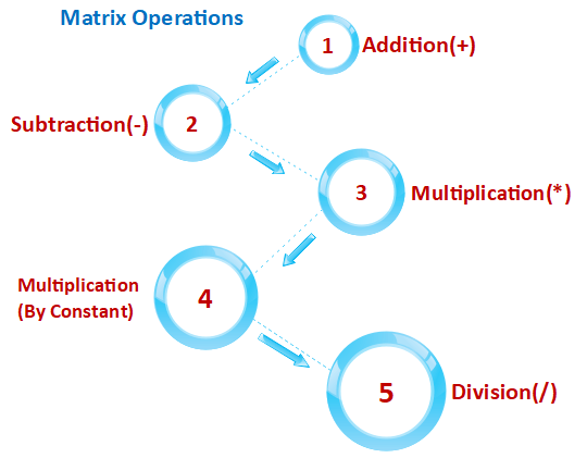
In R, we can perform the mathematical operations on a matrix such as addition, subtraction, multiplication, etc. For performing the mathematical operation on the matrix, it is required that both the matrix should have the same dimensions.

Let see an example to understand how mathematical operations are performed on the matrix.

Example 1

1. R <- matrix(c(5:16), nrow = 4,ncol=3)  
2. S <- matrix(c(1:12), nrow = 4,ncol=3)  
3.   
4. #Addition  
5. sum<-R+S  
6. print(sum)  
7.   
8. #Subtraction  
9. sub<-R-S  
10. print(sub)  
11.   
12. #Multiplication  
13. mul<-R*S  
14. print(mul)  
15.   
16. #Multiplication by constant  
17. mul1<-R*12  
18. print(mul1)  
19.   
20. #Division  
21. div<-R/S  
22. print(div)  

Output

      [,1] [,2] [,3]
[1,]    6   14   22
[2,]    8   16   24
[3,]   10   18   26
[4,]   12   20   28

      [,1] [,2] [,3]
[1,]    4    4    4
[2,]    4    4    4
[3,]    4    4    4
[4,]    4    4    4

      [,1] [,2] [,3]
[1,]    5   45  117
[2,]   12   60  140
[3,]   21   77  165
[4,]   32   96  192

      [,1] [,2] [,3]
[1,]   60  108  156
[2,]   72  120  168
[3,]   84  132  180
[4,]   96  144  192

      [,1]     [,2]      [,3]
[1,] 5.000000 1.800000 1.444444
[2,] 3.000000 1.666667 1.400000
[3,] 2.333333 1.571429 1.363636
[4,] 2.000000 1.500000 1.333333

Applications of matrix

1. In geology, Matrices takes surveys and plot graphs, statistics, and used to study in different fields.
2. Matrix is the representation method which helps in plotting common survey things.
3. In robotics and automation, Matrices have the topmost elements for the robot movements.
4. Matrices are mainly used in calculating the gross domestic products in Economics, and it also helps in calculating the capability of goods and products.
5. In computer-based application, matrices play a crucial role in the creation of realistic seeming motion.